The GreenStalk

“On any given Sunday, any team can beat any other team.”

-Bert Bell, NFL Commissioner, 1946-1959

We all love a good upset in sports.  That’s why the NFL famously embraces the fact that any team could beat another team.  But, this made me wonder: how does this compare across different sports?  Are some sports more or less prone to upsets (or, in other words randomness) than others?  I’m going to attack this question a couple ways.

Gini Coefficients

The first way to think about randomness in a sport is to look at how much inequality in wins there is between the good and bad teams.  Great win equality should correlate with more randomness in a sport, (since it’s harder for the genuinely good teams to consistently beat the worse teams).  And the most rigorous way to think about inequality is the Gini coefficient.

Gini coefficients are used by economists to measure inequality within a population.  Basically, you sort the population from poorest to richest, and plot the curve of their cumulative wealth (shown as the blue curve below).  You then compare that to a straight line (which would represent perfect equality).   The ratio of the area between the curves (the red striped area) to the total area (red plus blue) is the Gini coefficient.  So perfect equality would be a gini coefficient of 0, while perfect inequality would be a Gini coefficient of 1.0.

Figure 1: Illustrative Gini Coefficient

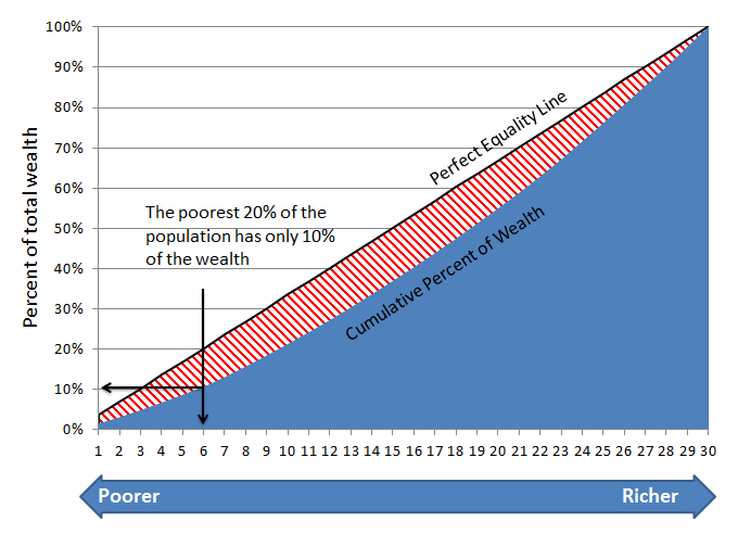
You may have noticed that the chart above has 30 points on the x-axis… that’s because these actually represent the 30 teams of the NBA, sorted by their 2010 win totals.  So, for example, the bottom six teams that year (Minnesota, Cleveland, Toronto, Washington, New Jersey, and Sacramento) had a total of just 10% of the league’s wins.

The actual Gini coefficient for the NBA that year, or the red area divided by the red + blue areas, is 0.175 (or 17.5%).  So, how does this compare to other sports?

Gini by Sport

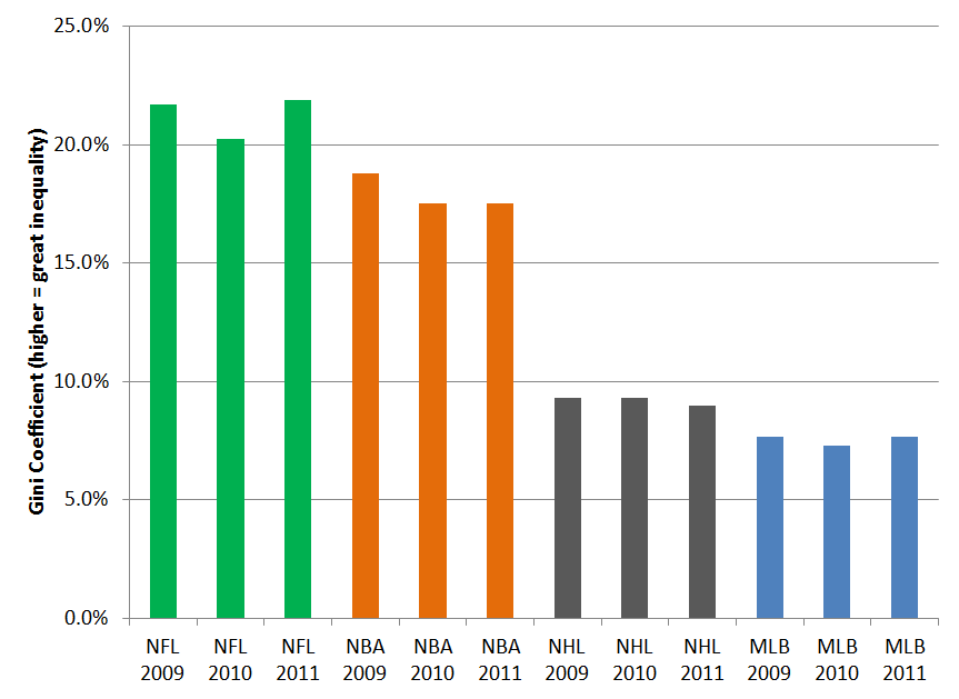
If we look at the Gini values by sport (see Figure 2 below), we can see a few interesting things.  First, they’re all pretty low – all below 25% (in contrast, the US income Gini coefficient is around 45%).  But there are also pretty significant differences between sports.  In fact, based on the past three years for each league, there isn’t ANY overlap between the ranges of values.  So there is the least disparity (indicative of more randomness) in baseball, followed by the NHL, then the NBA and finally, the most disparity / least apparent randomness in the NFL (ironic, given the claim about “Any Given Sunday”).

Figure 2: Gini Coefficients by Sport, Last Three Seasons

This analysis has a flaw, however.

Re-adjusting for Games Played

While they are really useful, Gini coefficients are particularly susceptible to measurement problems.  And I’ve discovered a weak spot here: each league plays a different number of games.  When you have a shorter season (like the NFL’s 16-game schedule), you have a greater chance for weird outlier events (e.g. win streaks from bad teams) to happen.  With more games, you have more mean reversion.

This can’t be corrected empirically (say, by dividing by the number of games).  But it is a perfect application for a Monte Carlo simulation, where you pull a smaller sample of games from the population, and re-calculate the Gini coefficients:

Figure 3: Games-Adjusted Gini Coefficients, based on Monte Carlo Simulations

Sampling smaller subsets of the MLB and NBA 2011 seasons, we can see that the Gini coefficients increase with fewer games, as expected.  In fact, The NBA Gini coefficient with 16 games is 22% – right in line with the NFL Gini coefficients.

Conclusion

So, it looks like baseball has more evenness between teams, based on the distribution of wins.  But in my next post, I’m going to look at this a different way, using a more head-to-head approach.