The GreenStalk

So, how much randomness is there in sports?

Last week I tried to answer this by looking at the differences between the win totals of the good and bad teams.  But that doesn’t tell the whole story, because it ignores who those wins came against.

Instead, it’s more interesting to ask the question: if one team is better than another, what is the probability that the better team wins?

Now, there’s no perfect way to define a “better team,” but we can use the team’s winning percentage as a decent estimate[1].  The difference between two teams’ winning percentages then gives us their mismatch in talent.  See the chart below (dashed lines indicate low base sizes):

It’s no surprise to see the lines going up and to the right – a bigger mismatch between teams should lead to greater odds of winning.

But the parity in the NHL and MLB is pretty striking.  This chart implies that in those sports, even in the most lopsided games, the stronger team could only be expected to win about 60% of the time[2].

This chart can also spur some interesting debates about why these charts look the way they do.  I don’t have the answers, but a few hypotheses:

1)      There is certainly some inherent randomness, which varies by sport.  I think this shows pretty conclusively that baseball and hockey have a greater proportion of randomness than football and basketball.

2)      The final score values also have some impact.  Consider that a typical hockey score is 2-1, versus a typical basketball score of 90-85.  A “point” in hockey often accounts for 50-100% of the team’s final score, while a “point” in basketball accounts for about 1% of the team’s final score.  When you have fewer scores happening in each game, this makes the outcome “lumpier”, and therefore more random.

Any other hypotheses?  Does this make you think about your favorite sports any differently?  Let me know in the comments.

“On any given Sunday, any team can beat any other team.”

-Bert Bell, NFL Commissioner, 1946-1959

We all love a good upset in sports.  That’s why the NFL famously embraces the fact that any team could beat another team.  But, this made me wonder: how does this compare across different sports?  Are some sports more or less prone to upsets (or, in other words randomness) than others?  I’m going to attack this question a couple ways.

Gini Coefficients

The first way to think about randomness in a sport is to look at how much inequality in wins there is between the good and bad teams.  Great win equality should correlate with more randomness in a sport, (since it’s harder for the genuinely good teams to consistently beat the worse teams).  And the most rigorous way to think about inequality is the Gini coefficient.

Gini coefficients are used by economists to measure inequality within a population.  Basically, you sort the population from poorest to richest, and plot the curve of their cumulative wealth (shown as the blue curve below).  You then compare that to a straight line (which would represent perfect equality).   The ratio of the area between the curves (the red striped area) to the total area (red plus blue) is the Gini coefficient.  So perfect equality would be a gini coefficient of 0, while perfect inequality would be a Gini coefficient of 1.0.

Figure 1: Illustrative Gini Coefficient

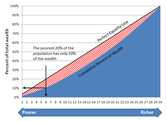
You may have noticed that the chart above has 30 points on the x-axis… that’s because these actually represent the 30 teams of the NBA, sorted by their 2010 win totals.  So, for example, the bottom six teams that year (Minnesota, Cleveland, Toronto, Washington, New Jersey, and Sacramento) had a total of just 10% of the league’s wins.

The actual Gini coefficient for the NBA that year, or the red area divided by the red + blue areas, is 0.175 (or 17.5%).  So, how does this compare to other sports?

Gini by Sport

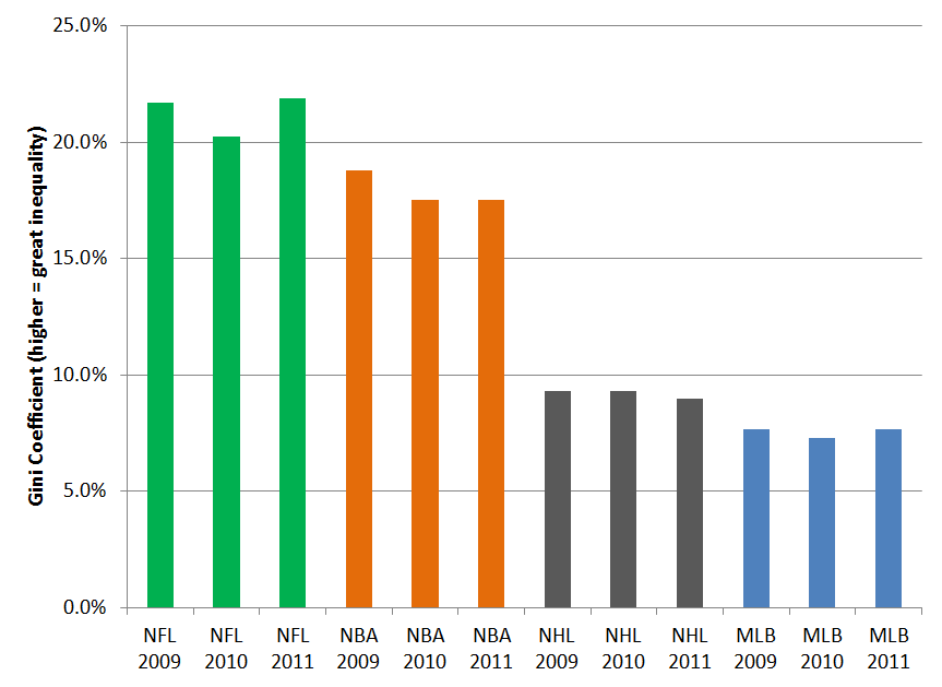
If we look at the Gini values by sport (see Figure 2 below), we can see a few interesting things.  First, they’re all pretty low – all below 25% (in contrast, the US income Gini coefficient is around 45%).  But there are also pretty significant differences between sports.  In fact, based on the past three years for each league, there isn’t ANY overlap between the ranges of values.  So there is the least disparity (indicative of more randomness) in baseball, followed by the NHL, then the NBA and finally, the most disparity / least apparent randomness in the NFL (ironic, given the claim about “Any Given Sunday”).

Figure 2: Gini Coefficients by Sport, Last Three Seasons

This analysis has a flaw, however.

Re-adjusting for Games Played

While they are really useful, Gini coefficients are particularly susceptible to measurement problems.  And I’ve discovered a weak spot here: each league plays a different number of games.  When you have a shorter season (like the NFL’s 16-game schedule), you have a greater chance for weird outlier events (e.g. win streaks from bad teams) to happen.  With more games, you have more mean reversion.

This can’t be corrected empirically (say, by dividing by the number of games).  But it is a perfect application for a Monte Carlo simulation, where you pull a smaller sample of games from the population, and re-calculate the Gini coefficients:

Figure 3: Games-Adjusted Gini Coefficients, based on Monte Carlo Simulations

Sampling smaller subsets of the MLB and NBA 2011 seasons, we can see that the Gini coefficients increase with fewer games, as expected.  In fact, The NBA Gini coefficient with 16 games is 22% – right in line with the NFL Gini coefficients.

Conclusion

So, it looks like baseball has more evenness between teams, based on the distribution of wins.  But in my next post, I’m going to look at this a different way, using a more head-to-head approach.

I’m a numbers guy – and the only things better than solar numbers are sports numbers.  So I’m going to reprieve my usual solar analysis for some sports analysis.

This year’s NFL season has a unique statistical race, as two quarterbacks (Drew Brees and Tom Brady) are on pace to break Dan Marino’s single-season passing record, and a third (Aaron Rodgers) is close.

Assessing the current stats

Both Brees and Brady are looking good for breaking Marino’s record.  Through 13 games, they have 4,368 and 4,273 yards respectively.  This puts them on pace for 5,376 and 5,259 yards each.  They’re comfortably ahead of the record pace, by 5.7% for Brees and 3.4% for Brady.

Another way to look at it: how many yards per game would they have to get in their final three games in order to just break Marino’s record?  For Rodgers, it’s 320 yards for each of his remaining three games.  For Brady, 270 yards per game.  Drew Brees only needs 239 yards per game from here on out.

So they look good now.  But I was still wondering whether there would be any other outside factors coming down the home stretch.  So I pulled some more data to test two more hypotheses.

Hypothesis 1: are their remaining opponents going to be tougher to gain yards on? 

Could it be true that these quarterbacks got to beat up on easier competition earlier in the season?  In fact, even if all else was equal, you would expect their past opponents to have given up more passing yards, just because they’ve already faced these record-setting passers.  And, more importantly, are their remaining competition going to be tougher to gain yards on?

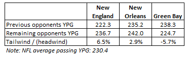
Happily for Brady & Brees, the answer is no.  Brady’s last three opponents (Den, Mia, and Buf) have given up, on average 236.7 passing yards per game.  This is 6.5% more than their previous opponents’ average.  Similarly, Brees’ three upcoming opponents have given up 2.9% more than his previous opponents.  So both of these guys are going to be facing slightly easier opponents down the stretch of their potentially record-setting run.

Unfortunately, Aaron Rodgers doesn’t have the same tailwind down the stretch.  His last three opponents (KC, Chicago, and Detroit) have given up 5.7% fewer passing yards per game than his previous opponents.

Passing Yards Per Game, Previous vs. Remaining Opponents

Hypothesis 2: Do passing yards fall over time? 

Is there any seasonality in passing yards?  There are a bunch of reasons to think there might be seasonal trends:

• As the weather gets worse, it’s tougher for the skill-based passing plays to be effective.
• Over time, defensive secondaries might get better, particularly for zone defenses which require coordination and discipline.
• On the other hand, as the season goes on, the timing of quarterbacks and wideouts might improve, particularly for timing-focused plays like slants and outs.

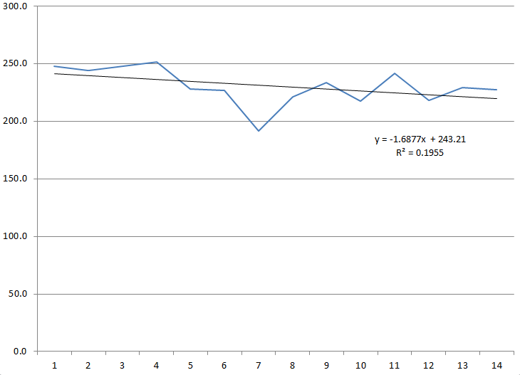
This year, through 14 weeks, there is a small downward trend in passing yards (see the chart below).  On average, the teams pass for approximately 1.7 fewer yards each week.  However, the R-squared value (.195) means that only about 20% of the weekly variation can be explained by the timing through the season.

Weekly Passing Yards per Game, 2011

If we look at the last few years, though, the seasonality appears even smaller:

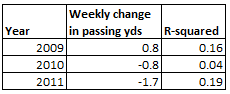
Weekly Passing Yards per Game – 2009, 2010, and 2011

When looking at all three years, the downward trend doesn’t seem as significant.  In fact, 2009 actually had a slightly positive change in passing yards over time (+0.8 yards per week), while 2010 was just a negative (0.8) passing yards per week.  It seems like there isn’t much seasonality to passing yards at all.

So all in all, it looks good for Brees and Brady.  Both are strongly ahead of the record pace, both have easier competition down the stretch, and it doesn’t seem like the colder weather at the end of the season will significantly reduce passing yards.  Now they just have to go out and play the games!